WebGPU Renderer: Transforms & Object Spaces

Controls

Overview

This is the second post in a series I am doing on creating my own renering engine using the WebGPU API. In this post I document everything I learned about transformations and object spaces while implimenting them into my rendering engine. You can see this in action in the interactive demo above.

Transforms

In the last post about the Graphics Pipeline, we not only saw a cool little triangle on the screen, but we also saw that the cool little triangle could rotate in little circles, which was pretty cool. The method in which I was rotating that triangle, however, was not very cool. You see, to achieve the rotation effect for the triangle, I was manually changing the position of each vertex in the triangle's vertex buffer. While this was okay for a single triangle doing a simple rotation, this method of manually moving vertices to different screen coordinates to achieve the impression of movement is not scalable at all once we want to see more complex shapes and models. Luckily for us, some really smart mathmaticians figured out a solution to this problem: transforms.

While you may not be familiar with the term 'transform', you almost certainly have utlized them before. Think about your favorite image editing software, such as Photoshop. In photoshop, you can place an image on a canvas. Once you've placed your image, there are three main ways you can transform this image. You move (translate) your image to a different part of the canvas, you can resize (scale) your image to be wider or taller, and you can rotate your image to be at a different orientation. These three types of transformations - translation, rotation, and scaling - are not only fundamental in 2D graphics but also form the main methods of object manipulation in 3D space. In 3D graphics, these transformations become more complex as they involve changes along three axes (X, Y, and Z) and are represented mathematically by transformation matrices. Each of these transformations can be visualized on the canvas above and we will explore how each of these transforms in 3D space can be represented by a specific type of matrix, allowing for precise and efficient manipulation of 3D models.

Scaling

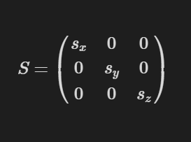
Scaling is the process of changing the distance between two respective points, essentially making an object bigger or smaller. This can be done independently on each axis. So, if we have a scaling matrix S and want it to scale by the components sx, sy, and sz, the object will be scaled by sx on the x-axis, sy on the y-axis, and sz on the z-axis. The actual values for the scaling matrix S would look like this: For example, if we applied this scaling matrix to our object: 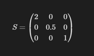it would be scaled by 2 on the x-axis, making it appear twice as wide, by 0.5 on the y-axis, making it appear half as tall, and would remain the same on the z-axis. A visualization of this happening in real time can be seen on the bottom row of triangles on the canvas above. The leftmost triangle is being scaled up and down on the x-axis, the middle triangle is being scaled up and down on the y-axis, and the rightmost triangle is being scaled on both the x and y axes simultaneously. Since the triangle is flat on the z = 0 plane, scaling it on the z-axis wouldn't have any visible effect.

Rotation

Rotation is the process of rotating an object around a given 3D axis by a certain amount of degrees through the origin. Imagine if you had your object and you stuck a rod through its center; that rod would represent the axis. By turning the rod, your object would rotate along with it by the same number of degrees. So, if we have a rotational matrix R and an angle theta, here are three possible matrix values for rotating along the x, y, and z axes respectively: 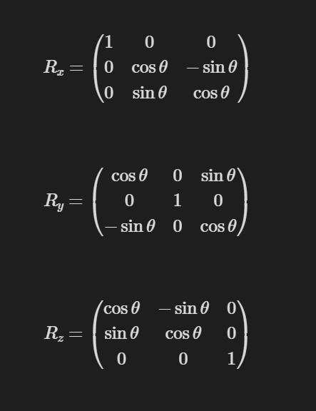Now, it's important to note that a rotation matrix can actually be described for any possible axis. However, the math behind this is substantially more complex and would require an understanding of something called Quaternions, which is a topic for another time. But just know that it is possible. You can visualize these rotations in real time by looking at the top row of triangles in our example. The leftmost triangle is rotating along the x-axis, the middle triangle along the y-axis, and the rightmost triangle along the z-axis.

Translation

Translation is the process of moving your object from one position to another. While this may seem like a straightforward operation, representing this transform introduces some challenges. The past two transformations we've looked at, scaling and rotation, are both linear transforms. A linear transform is a transform that maintains both the additive and scalar multiplication properties of vectors. In other words, if you have two vectors, and you apply a linear transform to each of them, and then add them together, it is the same as adding them together and then applying the transform. Similarly, if you have a vector, and you apply a linear transform to it, and then multiply it by a scalar, it is the same as multiplying the vector by the scalar and then applying the transform. As mentioned earlier, the rotation and scaling transforms meet these requirements, and the benefit of this is that they can be represented with 3x3 matrices. However, the translation transformation, while maintaining additivity (vector addition), does not maintain the property of scalar multiplication in the way linear transformations do. This is because translating a vector does not keep the origin fixed; for instance, translating the zero vector results in a non-zero vector. Therefore, translation is not a linear transformation and cannot be represented by a 3x3 matrix. This presents a challenge because we want to represent any given transformation by a single matrix, and our current method of doing that with 3x3 matrices will not work for translations. Don't worry though, because once again, some genius mathematicians have saved us. If we instead describe our transformations in 4 dimensions instead of 3, we can actually create a single matrix capable of performing all three kinds of transformation. This is known as an affine transformation. So, if we want to move our object by the values tx in the x direction, ty in the y direction, and tz in the z direction, we can create a translation matrix T with the following values: As you can see, the amounts we want to translate our object by are stored in the last column of the matrix. The top left 3x3 values are just the identity matrix, which keeps the scale and orientation of the object constant. You may also notice that we now also have a new bottom row in our matrix with the values [0,0,0,1]. This is just there to make the new matrix have uniform dimensions and definitely will not come into play later **winks slyly** **grins** .

You should also note that the previous transform matrices discussed earlier should be turned into affine transformations; this can easily be done by just adding a row and column, with 0s for the translation values in the last column, and the bottom row containing the values [0,0,0,1]. Also, when using these matrices to translate a point, because we are now working with 4-dimensional matrices, our 3D points will also need a 4D representation. This is done by taking some point [x,y,z] and changing it to [x,y,z,1].

Translation can be seen in real-time with the middle row of triangles, where the leftmost triangle is moving side to side on the x-axis, the middle triangle is moving up and down on the y-axis, and the rightmost triangle is moving back and forth on the z-axis.

Transform Concatination

The beauty of these transforms is that any series of transformations applied to an object can actually be represented by a single transformation matrix. A single transformation matrix can apply a scale, rotation, and translation transformation! This combined transformation matrix can be obtained by multiplying several transformation matrices together. Be careful, though, because matrix multiplication is noncommutative, meaning that the order in which you perform the multiplication matters and will yield different results. The way I think about it is that the order in which the transformations are applied happens from right to left. So, for example, if you had three transformation matrices M1, M2, M3, and you wanted to create a concatenated matrix M that applied M2, then M3, then M1, you would do M = M1 * M3 * M2.

Object Spaces

Okay, so we've laid out this framework for how we can represent our transforms, but how should we actually use them? Here, I will introduce to you the idea of object spaces. Object spaces are different coordinate systems in which our objects can exist. Remember, we have been talking about our virtual objects as if they really exist in some 3D virtual world, but at the end of the day, the screen on which we view them is two-dimensional. These different object spaces exist in order for us to control the way in which our objects in virtual 3D space will appear on our 2D screen. The different object spaces that we will look at are Model space, World space, Eye space, and Perspective space.

Model Space

Model space is the initial coordinate space in which a 3D model exists. In this space, the position of each vertex is defined only in relation to the other vertices that make up the model, making the object itself the center of its own universe. This space is typically moat important to the person designing the 3D model, as it's where they determine the object's shape, size, and the relative positioning of its vertices. In a real-world example, imagine a teapot. The teapot could be considered in Model space when it is still a drawing in the designer's sketchbook. Here, the designer has laid out the shape of the teapot, the proportions of the spout, the shape of the handle, etc. Because this is the default space for a model, no transformation matrix needs to be applied to it to reach this space. It is its default space.

World Space

World space is the coordinate system of the actual virtual world. In world space, an object's vertex coordinates are in relation to the world that it currently exists in. This is somewhat analogous to our real world, where each object has coordinates that define its location within the world. Going back to the previous example, let's say you pick up a teapot from the teapot factory and want to place it in your room. Here, you can think of your room as the world. Once you place your teapot in your room at a certain position and orientation, you have transformed that teapot from model space to world space, as it now has a position within your room. 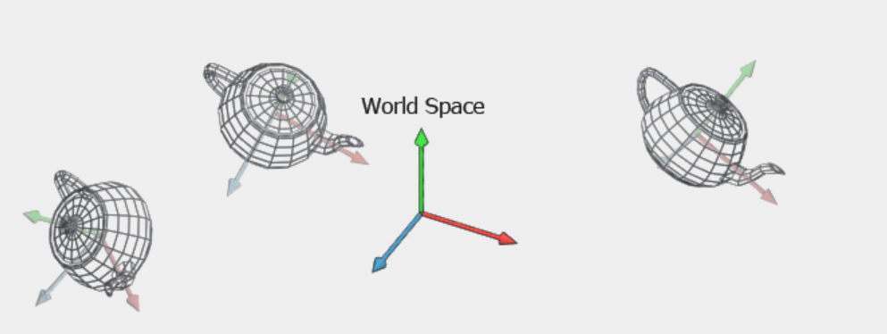The object's vertex coordinates have gone from only being in relation to each other, to now being in relation to every other object in the room. In our graphical applications, the way we actually take an object in model space and bring it into world space is with the transforms we discussed in the previous section. Within any given world, an object can have a position, rotation, and scale. We know that each of these transformations can be applied with their own transformation matrix, and any given series of transformations can be represented by a single transformation matrix. Therefore, our goal is to create a single matrix that can transform an object from model space to its given translation, rotation, and scale in world space. Also, remember that the order in which we multiply these matrices is important to receive the results we want. The most intuitive way to apply these transforms is first to scale, then rotate, then translate. This order of transforms is known as the TRS matrix, and this TRS matrix is what we use to transform our model from model space to world space.

Eye Space

So now that we have a representation of our objects and their positions within our virtual world, our next step is to define how we want to view this world. This process begins by converting everything into eye space, also known as camera space or view space. Eye space is the coordinate system where everything is positioned relative to the viewer, similar to how we perceive the world relative to our eyes. In our teapot example, this would be the teapots position relative to us when we are standing in the room viewing it. In this space, the virtual world is viewed from the camera's perspective. 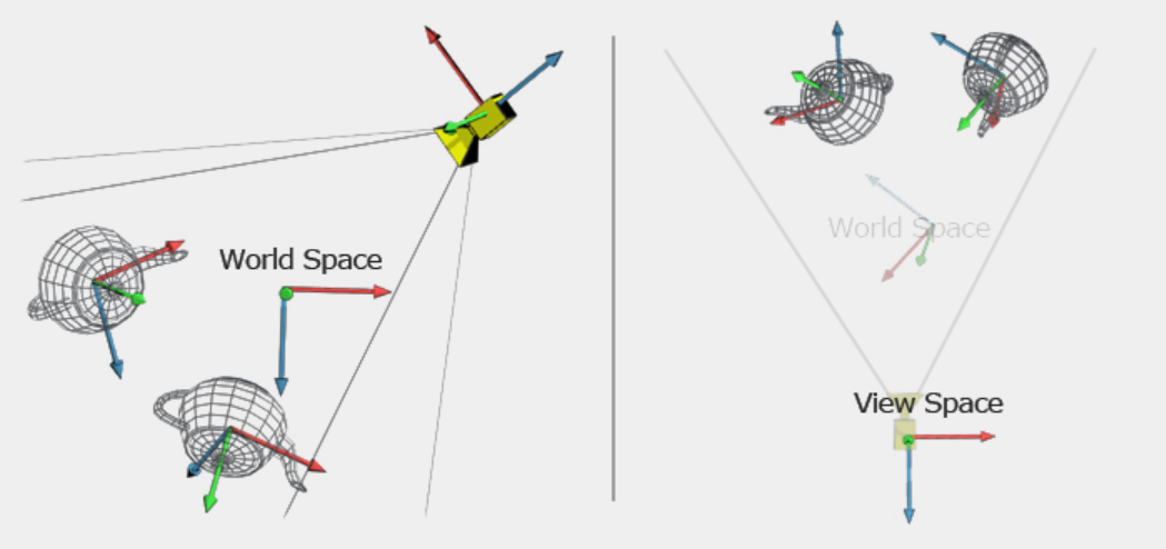The camera, like any object in the virtual world, has a position and rotation, and while it also has a scale, this is typically ignored as it shoudln't have an influence on the way in which we are viewing the scene. Our goal is to make the camera the reference point of the world, meaning all objects' positions become relative to the camera's location and orientation. This is achieved by transforming each object in world space using the inverse of the camera's TRS matrix. Applying this inverse transformation aligns the entire scene to the camera's viewpoint, effectively repositioning the world as if the camera were at its origin.

Perspective Space

Now that all of the objects in our scene are positioned in relation to the camera, our next step is to project every vertex onto the viewing plane. You can think of this as if you were taking a picture of your teapot in your room. All of the 3D objects that are visible in your room are projected onto an image plane (the photograph). We need to do the same thing with our virtual 3D scene. We need to take all the data in our 3D scene and project it into a 2D space so we can actually view it on our screen. If we assume that our camera is located at the origin, our x-axis points right, our y-axis points up, and our camera is looking down the positive z-axis, a naive solution to this problem would be to just take each object's x and y coordinate and find its corresponding pixel. While this solution may allow you to view a distorted image of the scene, it is ignoring crucial elements of projection that are crucial for our scene to look realistic: perspective, as well as the field of view (FOV) and the aspect ratio of the viewing plane. Perspective is something that is ever-present in our view of the world, yet we sometimes take it for granted because our brain does all the hard work for us automatically. What perspective is, is the effect of objects that are farther away look smaller, and objects that are closer look larger. The FOV determines the extent of the observable world seen at any moment, and the aspect ratio ensures that the x and y dimensions are proportionally correct on our screen. 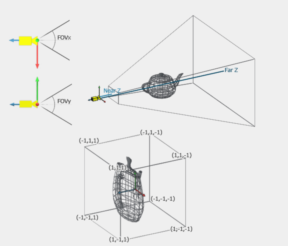In order to compute this, we need to be able to scale a given vertex's x and y components by its 1/z component. Unfortunately, though, this scale on only the x and y components is not possible with our 4x4 matrix! Oh no! But hey, don't worry. Because once again, those mathematicians came up with a genius solution to save us. This time, the solution is known as homogeneous coordinates. Remember earlier we said that we make our 3D points 4D by just adding a 'useless' 1 at the end? Well, it turns out that extra number on the end is not useless after all. That extra number on the end is what we use for perspective division, meaning that each of the first three components of our point is divided by the fourth component. This is what allows us to view perspective in our final render.

Resources

Real-Time Rendering 4th Edition - Tomas Akenine-Moller et al.
World, View and Projection Transformation Matrices - Coding Labs
The Math behind (most) 3D games - Brendan Galea